Deep Differentiable Logic Gate Networks: An Intro
This is meant to be a readable intro to the 2022 paper on Deep Differentiable Logic Gate Networks by Petersen et al.
This is the original paper. My implementation of the paper is available here.
DDLGNs?
Idea. At inference time, neural networks rely on floating point matrix multiplications, which is expensive and time-consuming, more so than, say, logic gate networks (LGNs).
Problems. LGNs are discrete and non-differentiable, and so we cannot train them with gradient descent.
DDLGNs!
Definition. Deep Differentiable Logic Gate Networks (DDLGNs) are LGNs made trainable through differentiable relaxations during training.
We replace all 16 possible binary logic gates with their probabilistic real-valued analogues (e.g. with ) to make them differentiable.
Training
In a DDLGN, we want to learn a categorical probability distribution over the choice of logic gate at each neuron. So each neuron is parameterized with 16 weights which are softmaxed to the probability simplex.
Note that unlike a fully-connected network, in a DDLGN each neuron accepts only two inputs.
Forward Pass. Let be the probability of each gate, be the respective real-valued relaxation, and be the inputs to our neuron. We compute a weighted sum w.r.t. each of the 16 gates to obtain the activation :
As training progresses, the categorical probability distribution eventually collapses to a single gate, which we can use for quick inference.
Backward Pass. Let the loss function be . For a single node, we want to know for each weight the gradient . By the chain rule:
Now we derive an expression for the second gradient. From the forward pass expression:
Recall that , so the gradient is obtained by picking the entry from the Jacobian of the softmax function. Briefly, the softmax function is a vector-valued function that maps the tuple to the tuple . The entry of its Jacobian is given by where is the Kronecker delta.
Remark. I will not discuss here how this expression for each entry of the Jacobian is obtained. This article is a good resource for the complete derivation.
Applying this result, we get:
Simplifying:
Recall that this last term is our original activation . We get:
This is a very elegant result and it makes intuitive sense! We can see that the change in the loss due to depends on how much the weighted sum () disagrees with the gate's real-valued relaxation (), scaled by how much our DDLGN believes in the gate ().
Inference
This is really the whole point of the architecture. After training, each neuron's categorical distribution over the 16 gates is discretized and the network picks the single most likely gate, i.e. .
So what remains is a regular logic circuit with simple boolean inputs (the authors use binarized MNIST, for instance). We don't have to deal with matrix multiplications or floating point numbers at all or any of that other clunky stuff. The paper reports over a million MNIST images classified per second on a single CPU core. The memory footprint is also tiny (each neuron's gate choice can be stored in just 4 bits, since there are only 16 possibilities, and the random connections don't even need to be stored explicitly as they can be regenerated from a single seed).
We can't have nice things
Training a DDLGN is, sadly, more expensive than training a comparably-accurate conventional neural network, because at every neuron we must evaluate all 16 relaxed gates on every pass. The paper argues that this is an acceptable trade-off, since for edge and embedded deployment, training happens once, offline, while inference happens constantly, and on hardware where every bit of compute and memory counts.
Implementation & Results
I implemented from scratch a minimal version of a DDLGN in PyTorch. My code is available here.
My DDLGN was trained on binarized MNIST with the following config taken from the original paper:
| Hyperparameter | Value |
|---|---|
| Layers | 6 |
| Neurons per layer | 8,000 |
| Batch size | 100 |
| Learning rate | 0.01 |
| Softmax temperature (τ) | 10 |
| Epochs | 10 |
Note that the authors train all their models for 200 epochs, but I chose 10 in the interest of saving time.
My results are below:
| Metric | Value |
|---|---|
| Soft (pre-discretization) test accuracy | 96.79% |
| Hard (post-discretization) test accuracy | 96.26% |
| Discretization gap | 0.53% |
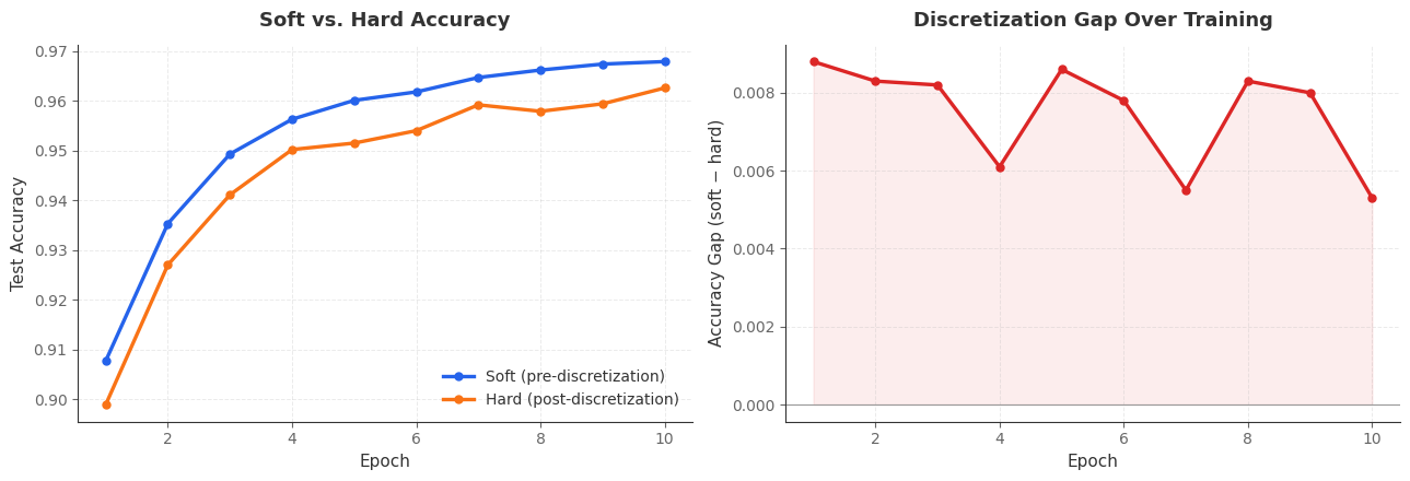
This discretization gap is somewhat larger than the paper's reported figure of < 0.1%, which makes sense given the far shorter training run. The discretization gap depends on how much each neuron's softmax distribution has committed to a single gate, which continues well past epoch 10. Tracking the gap across epochs, we see a marked decrease in the discretization gap:
It's also worth looking at what the network actually learned at the gate level. Below is the distribution of learned logic gates across all neurons in the first and last layers:
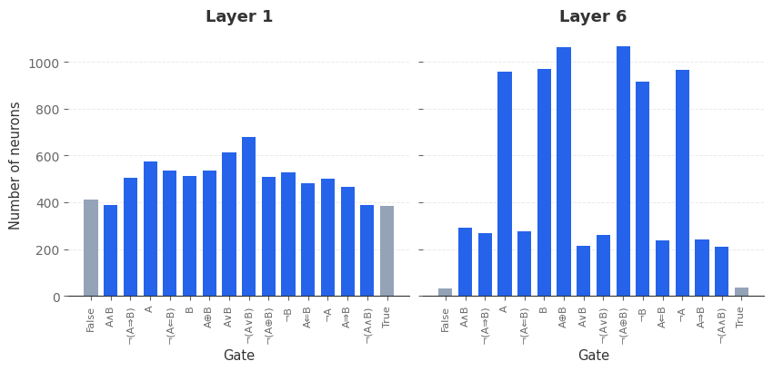
As expected, the first layer's gate distribution is diverse, while the last layer's is concentrated, with the constant true/false gates having almost vanished.